Tutorial A : Single Qubit Operations and Visualization of the Qubit State
Contents
Tutorial A : Single Qubit Operations and Visualization of the Qubit State
Tip
Remember, to interact with the code in this Quantum Programming tutorial, go over to the ‘rocket’ icon on the top right of your page and select “Live Demo”. From there, you’ll be able to rerun the code cells individually and edit the code.
Objectives:
to explore single-qubit gate operations.
to visualize a single-qubit state.
For this first tutorial, we will apply quantum gates to a singular qubit to observe their effects on the qubit’s state.
We will need to build a quantum circuit. To do so, we are using the Qiskit software development kit or simply Qiskit which allows us to do quantum circuit computation in the Python programming language and access the backend of IBM simulators and quantum devices.
1. Importing Qiskit SDK into our Python Editor
By running the following programming code, we will be able to use Qiskit for the rest of the tutorial.
import qiskit
from qiskit import *
qiskit.__version__ # This tells us which version of Qiskit we have
'0.19.2'
With Qiskit imported, we can now use its built-in functions to build our circuit.
2. Creating a Quantum Circuit with One Qubit
To create a circuit, we use the QuantumCircuit() function. In the parentheses (), we will insert the number of qubits that we wish to have. In this case, we desire only one so we put:
myquantumcircuit= QuantumCircuit(1) # You can label your quantum circuit anything.
Above, we’ve called our quantum circuit myquantumcircuit and given it a single qubit. Now, let’s draw our circuit to see what it looks like by using the draw() function.
myquantumcircuit.draw(output='mpl')

Great! We have our first quantum circuit and it’s that simple!
In order to make useful circuit however, we’ll need to perform operations, like adding a quantum gate and measuring to see what the qubit’s state is. So let’s do that now.
3. Applying a Quantum Gate
There are several gates that we can add to our circuit. But let’s start with a simple one.
For now we can apply an X gate which changes the state of our qubit to ‘1’ if it is initially ‘0’ and to ‘0’ if it is initially ‘1’.
Note
If you know about logic gates, it is analogous to the NOT gate.
The x() function applies an X gate. Note that the 1st qubit in a circuit is label as the 0th qubit, hence we use x(0) to apply the X gate to the first qubit.
myquantumcircuit.x(0)
myquantumcircuit.draw(output='mpl')
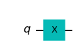
We’ve drawn our circuit at once to see what it looks like, and now we see a box with an ‘X’ added onto our qubit.
The next step is to know what this gate does to the state of our qubit. For this we’ll need to measure the circuit.
4. Measurement of a Quantum Circuit
Measurement is necessary to extract information from our system. But remember, when we measure a quantum system, it collapses to a classical state so that we may no longer be able to perform quantum computation on said system. For this reason, we leave measurement as the very last step to our quantum circuit.
To measure, we will need to add a classical bit to “collect” the information from the quantum bit.
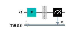
When we apply measure_all() and then draw(), the final circuit shows an analog scale icon with an arrow point to a new double line which appears below our first qubit.
myquantumcircuit.measure_all()
myquantumcircuit.draw(output='mpl')
However, we still do not know what our measurement is. This is because we haven’t run our quantum circuit!
All we have done until this point is to design a circuit to be run on a quantum computing device or a simulator.
So now we have to establish a connection to a quantum computer or simulator to get our results.
5. Connecting to an IBM Quantum Device or Simulator.
IBM allows us to access some quantum computers and quantum simulators for free in the cloud. To find out which IBM quantum devices and simulators are available, click here.
Note
Simulators are classical hardware made to mimic quantum hardware.
We’ll use the Python-based 'qasm_simulator' and we’re calling it sim for short.
sim = BasicAer.get_backend('qasm_simulator')
Once we’ve defined our sim, let’s go ahead and execute() our quantum circuit.
job=execute(myquantumcircuit,sim,shots=1)
But where are the results?
We have definitely run the circuit, but we need new functions to display the results…
6. Getting Results
If we call the simply call .result(), it looks like this.
job.result()
Result(backend_name='qasm_simulator', backend_version='2.1.0', qobj_id='5a046ba6-b30c-47be-a501-70e011512f7c', job_id='fb6df446-2f35-4a80-90cd-91808ce25096', success=True, results=[ExperimentResult(shots=1, success=True, meas_level=2, data=ExperimentResultData(counts={'0x1': 1}), header=QobjExperimentHeader(clbit_labels=[['meas', 0]], creg_sizes=[['meas', 1]], global_phase=0.0, memory_slots=1, metadata={}, n_qubits=1, name='circuit-0', qreg_sizes=[['q', 1]], qubit_labels=[['q', 0]]), status=DONE, name='circuit-0', seed_simulator=353647172, time_taken=0.0)], status=COMPLETED, status=QobjHeader(backend_name='qasm_simulator', backend_version='2.1.0'), time_taken=0.0)
Above tells us quite a lot, incltuding the job id, whether the job was successful, time taken and many more details.
To simplify, we’ll simply use result().get_counts() and print() to extract the result from job.
myresult=job.result().get_counts()
print(myresult)
{'1': 1}
Our result reads that we measured the state '1' once for our qubit.
Let’s try running the circuit more than once. To do this, we change the number of shots in our execute() function. We’ll run the circuit 50 times with shots=50.
multi_job=execute(myquantumcircuit,sim,shots=50)
myresult=multi_job.result().get_counts()
print(myresult)
{'1': 50}
Now we see that we got the result ‘1’ each time.
This is expected as Qiskit initializes qubits in the state ‘0’ unless we specify it to initialize in another state. Then we applied an X gate which flipped our qubit from the ‘0’ state to the ‘1’ state.
There’s nothing too interesting right now, but let’s find another way to visualize our results.
7. Visualizing Results
We can plot histograms of our results by using another module from Qiskit. We’ll import the module now.
from qiskit.visualization import *
The module qiskit.visualization is imported. Now we can plot the histogram.
plot_histogram(myresult)
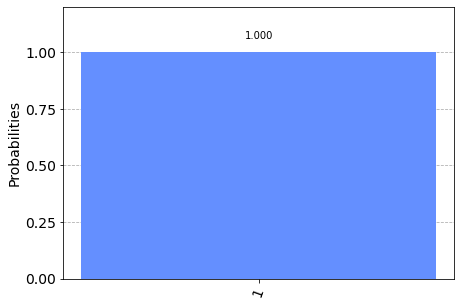
Super! We now have a histogram of our result. The histogram is clear that we got the state ‘1’ with 100% probability.
There are other cool ways to plot our results, but for that we’ll need to use the backend of the statevector_simulator instead. We’ll do this in later tutorials when we have a more interesting circuit.
Let’s try something else… Here’s a cool way to see what happens to our qubit using the Bloch sphere representation.
myquantumcircuit2= QuantumCircuit(1) # Recreating the same circuit with 1 qubit
myquantumcircuit2.x(0) # Recreating the circuit by adding an X gate
visualize_transition(myquantumcircuit2, trace=True, saveas=None, fpg=50, spg=2)
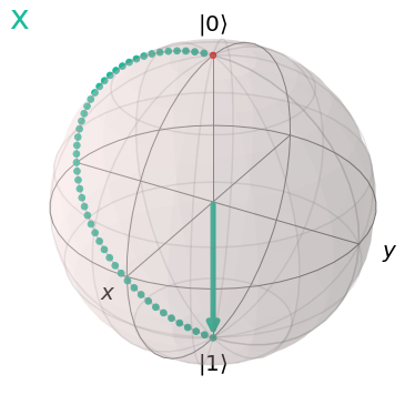
Cool! The state of our qubit went from \(|0\rangle\) to \(|1\rangle\) by rotating \(180^\circ\). Let’s look at some more interesting quantum gates.
8. Playing with Superposition
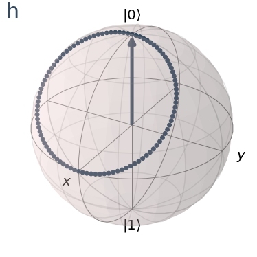
A gate that we definitely need to take a look at is the gate that creates a superposition. It’s called a Hadamard gate and we use the function h() to apply it to a qubit.
Let’s apply it now.
superpositioncircuit=QuantumCircuit(1) # Make a circuit with 1 qubit
superpositioncircuit.h(0) # Apply Hadamard gate
superpositioncircuit.draw(output='mpl') # draw circuit
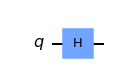
Right, now we have a new circuit with a ‘Hadamard’ gate. Let’s visualize what happens to the qubit.
visualize_transition(superpositioncircuit, trace=False, saveas=None, fpg=50, spg=2)
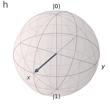
Did you see that?
The qubit did not go all the way to the state \(|1\rangle\). It stopped midway between. This is our superposition state of \(|0\rangle+|1\rangle\). It’s in both \(|0\rangle\) and \(|1\rangle\) at the same time.
But let’s see what happens when we measure the circuit…
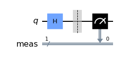
superpositioncircuit.measure_all() # Do the measurement on all qubits
superpositioncircuit.draw(output='mpl') # Draw the circuit
superpositionjob=execute(superpositioncircuit, sim, shots=100) # Execute the circuit with 100 shots
superpositionresult=superpositionjob.result().get_counts() # Get the result
print(superpositionresult) # Print the result
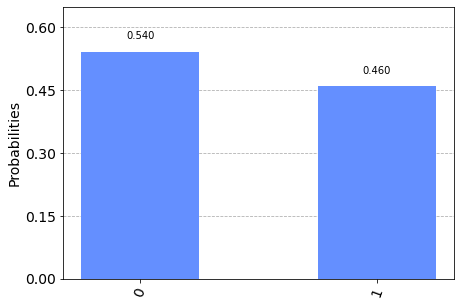
{'1': 46, '0': 54}
When we measured our circuit, we got two possible results: the \(|0\rangle\) state and the \(|1\rangle\) state. This is because when we measure a superposed state, the qubit “chooses” between one of the measurable states. For our 100 executions of the circuit, we should get a fairly equal split, about 50-50 for the \(|0\rangle\) and \(|1\rangle\) states.
Tip
Try rerunning the above code cell again and see if you get a slightly changed result.
An now to plot the histogram…
plot_histogram(superpositionresult)
9. Applying More than One Gate
Let’s now apply more than one gate to the same qubit.
moregates=QuantumCircuit(1)
moregates.x(0)
moregates.h(0)
moregates.draw(output='mpl')
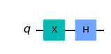
We’ve applied an X gate followed by a Hadamard gate.
visualize_transition(moregates, trace=True, saveas=None, fpg=50, spg=2)
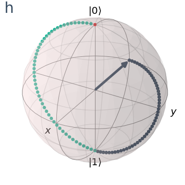
From above, we see two transitions. The first transition shows the flip of the qubit’s state from \(|0\rangle\) to \(|1\rangle\), after which the second transition takes the qubit from \(|1\rangle\) to an equal superposition state. This state is slightly different to the superposition state that we saw previously. In fact, what we saw before was the \(|0\rangle + |1\rangle \). What we see right above is the \(|0\rangle -|1\rangle\) state.
Note
The Hadamard gate takes a qubit in state \(|0\rangle\) to the superposed state \(|0\rangle + |1\rangle\). On the other hand, the Hadamard gate takes a qubit in state \(|1\rangle\) to the superposed state \(|0\rangle - |1\rangle\).
moregates.measure_all() # We must measure first before executing
job=execute(moregates, sim, shots=100)
counts= job.result().get_counts()
plot_histogram(counts)
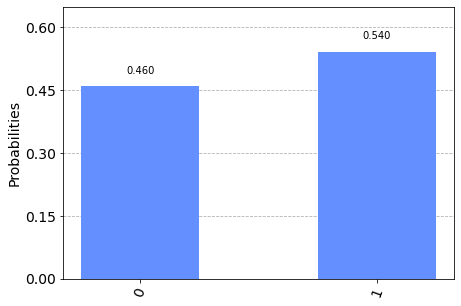
By executing the circuit, we see that there is no measurable difference between the \(|0\rangle - |1\rangle\) state and the \(|0\rangle +|1\rangle\) state from before. At least not using this measurement basis…
10. Applying the Same Gate Twice
Something interesting occurs when we apply some gates twice. Let’s see.
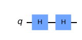
samegatetwice= QuantumCircuit(1)
samegatetwice.h(0)
samegatetwice.h(0)
samegatetwice.draw(output='mpl')
visualize_transition(samegatetwice, trace=True, saveas=None, fpg=50, spg=2)
Hmmm
How about if we started from the state \(|1\rangle\) and applied the Hadamard twice.
samegatetwice2=QuantumCircuit(1)
samegatetwice2.x(0) # flipping to state 1 first
samegatetwice2.h(0)
samegatetwice2.h(0)
visualize_transition(samegatetwice2, trace=True, saveas=None, fpg=50, spg=2)