Tutorial B: More Single Qubit Gates

Tutorial B: More Single Qubit Gates¶

In this short tutorial, we’ll cover more quantum gates.

Objectives:¶

to apply the two other Pauli Gates.
to apply gates with parameters and other phase gates.

Importing Modules

from qiskit import *
from qiskit.visualization import *

In Tutorial A, we covered only two: the X gate and the Hadamard gate. There are more quantum gates to explore, so let’s go through a few ones now.

1. Pauli Gates¶

The X gate is grouped with two other gates, namely the Y gate and the Z gate. Together with the Identity operator, these are called Pauli gates. We will test these out now.

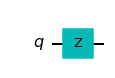
ycircuit=QuantumCircuit(1)
ycircuit.y(0)
ycircuit.draw(output='mpl')

Above, we’ve created a quantum circuit with a Y gate. Let’s visualize what happens.

visualize_transition(ycircuit, trace=True, saveas=None, fpg=25, spg=2)

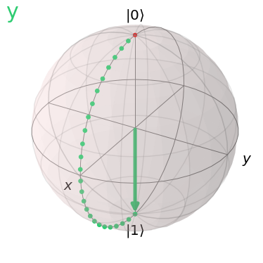
Let’s compare to the X gate that we had before.

xcircuit=QuantumCircuit(1)
xcircuit.x(0)
visualize_transition(xcircuit,trace=True, saveas=None, fpg=25, spg=2)

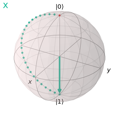
Well, we see that the qubit state goes from \(|0\rangle\) to \(|1\rangle\) when both gates are applied. There’s just one difference… The trace the vector makes in the transition.

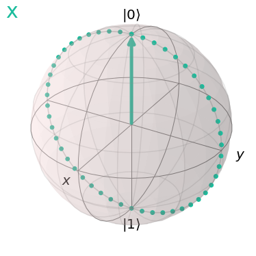
Let’s verify this by applying each gate twice.

xcircuit=QuantumCircuit(1)
xcircuit.x(0)
xcircuit.x(0)
visualize_transition(xcircuit,trace=True, saveas=None, fpg=25, spg=2)

ycircuit=QuantumCircuit(1)
ycircuit.y(0)
ycircuit.y(0)
visualize_transition(ycircuit,trace=True, saveas=None, fpg=25, spg=2)

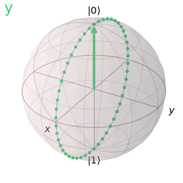
You may have noticed that the X gate causes a rotation about the x axis, whilst the Y gate causes a rotation about the y axis.
Let’s examine the Z gate now.

zcircuit=QuantumCircuit(1)
zcircuit.z(0)
zcircuit.draw(output='mpl')

visualize_transition(zcircuit, trace=True, saveas=None, fpg=25, spg=2)

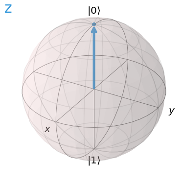
You’ll notice no transition as the measurement axis for the qubit states \(|0\rangle\) and \(|1\rangle\) are on the z axis. A rotation about the z axis would mean that the vector is spinning on itself.

To visualize a transition with the Z gate, we’ll place the qubit state at an angle. We’ll use the Hadamard to place the qubit in superposition, then apply the Z gate.

zcircuit=QuantumCircuit(1)
zcircuit.h(0)
zcircuit.z(0)
zcircuit.draw(output='mpl')

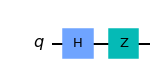
visualize_transition(zcircuit, trace=True, saveas=None, fpg=25, spg=2)

The light blue trace represents the z axis rotation.
Great! We’ve seen two more gates.

Short Quiz¶

Can you think of a sequence of two gates that will allow the qubit to end up in the same state as above?

Test it out in the space below then click to reveal the answer.

test_circuit=QuantumCircuit(1)

# Write your code here to add two of the four gates that we've learnt to the quantum circuit # 

# visualize_transition(test_circuit, trace=True, saveas=None, fpg=25, spg=2)  #Remove the first '#' on this line

Answer: Apply first the X gate followed by the Hadamard gate to get the \(|0\rangle -|1\rangle\) state.

2. Other Gates¶

Coding Exercise # 1¶

Use the space below to test the following gates: the S gate with s() and T gate with t().

Hint:

Try applying a certain gate before to be able to visualize a transition for the s and t gates.

scircuit=QuantumCircuit(1)

# Write code to visualize the S gate transition #

#visualize_transition(scircuit, trace=True, saveas=None, fpg=25, spg=2)  #Remove the first '#' on this line

tcircuit=QuantumCircuit(1)

# Write code to visualize the S gate transition #

#visualize_transition(tcircuit, trace=True, saveas=None, fpg=25, spg=2)  #Remove the first '#' on this line

What you should see:

After placing the qubit in equal superposition you shall see that the S gate causes a 90\(^\circ\) rotation about the z axis, whilst the T gate causes a 45\(^\circ\) rotation about the z axis.

Coding Exercise #2¶

The S and T gates above aren’t like the gates we’ve encountered previously which act as their own inverse. The reverse operations corresponding to these two gates are: \(S^\dagger\) and \(T^\dagger\) respectively. The ‘ \(\dagger\) ‘ symbol is called ‘dagger’. Try visualizing the sdag() and tdag() operations in the cell below.

dagger_circuit= QuantumCircuit(1)

# 1. Write code to place the qubit in equal superposition

# 2. Write code to apply an S or T gate #

# 3. Write code to apply the corresponding reverse gate

#visualize_transition(dagger_circuit, trace=True, saveas=None, fpg=50, spg=2)  #Remove the first '#' on this line

3. Parameterized Gates¶

All the gates covered so far show specific angles of rotation about the x, y and z axes. How about we take a look at some that the user defines. These are called parameterized gates since they require an input angle parameter.

Here are some single-qubit parameterized gates:

The Rotation X gate rx() applies a rotation about the x axis
The Rotation Y gate ry() applies a rotation about the y axis.
The Rotation Z gate rz() applies a rotation about the z axis.
The Rotation gate r() applies a vertical rotation and a horizontal rotation.

Let’s apply some parameterized gates.

import numpy as np    # Importing numpy

angle_in_degrees= 120

theta= angle_in_degrees * np.pi/180 

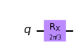
param_circuit=QuantumCircuit(1)

param_circuit.rx(theta,0)  # We apply a rotation of theta to the first qubit. 

param_circuit.draw(output='mpl')

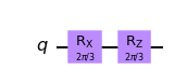
param_circuit.rz(theta,0)
param_circuit.draw(output='mpl')

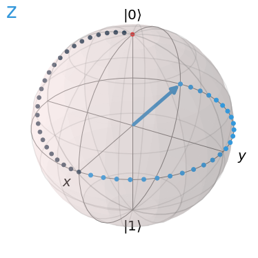
visualize_transition(param_circuit, trace=True, saveas=None, fpg=25, spg=2)

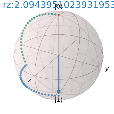
There you go!
We’ve shown how quantum gate operations can allow us to transition a qubit’s state to just about anywhere on the Bloch Sphere.
This is precisely what gives quantum computation an advantage. Information is no longer processed as solely ‘0’ or ‘1’ but rather in superposition of ‘0’ and ‘1’ in a complex state space!

Try Your Own Code¶

We leave you this space to enter and play around with your own quantum programming code. You may want to restart the kernel.

import qiskit 
from qiskit import *
from qiskit.visualization import *
import numpy as np 

Tutorial A : Single Qubit Operations and Visualization of the Qubit State

Tutorial C: Multi-Qubit States

World of Tech